BYOM, byom_snail_embryo.m, DEBkiss with Lymnaea
- Author: Tjalling Jager
- Date: April 2017
- Web support: http://www.debtox.info/byom.html
- Back to index walkthrough_debkiss_paper.html
BYOM is a General framework for simulating model systems in terms of ordinary differential equations (ODEs). The model itself needs to be specified in derivatives.m, and call_deri.m may need to be modified to the particular problem as well. The files in the engine directory are needed for fitting and plotting. Results are shown on screen but also saved to a log file (results.out).
The model: DEBkiss following Jager et al (2013), http://dx.doi.org/10.1016/j.jtbi.2013.03.011.
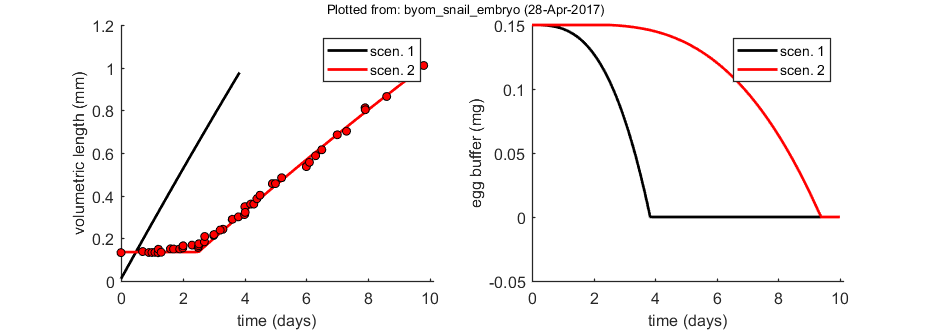
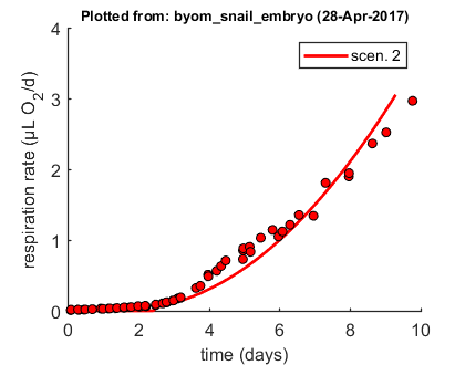
This script: The case study in the original DEBkiss paper for the pond snail Lymnaea stagnalis. This is the embryonic development. Data from Horstmann (1958). There is no fitting in this script.
Contents
Initial things
Make sure that this script is in a directory somewhere below the BYOM folder.
clear, clear global % clear the workspace and globals
global DATA W X0mat % make the data set and initial states global variables
global glo          % allow for global parameters in structure glo
global pri zvd      % global structures for optional priors and zero-variate data
global DATAx Wx     % optional global for extra data set with different x-axis
diary off           % turn of the diary function (if it is accidentaly on)
% set(0,'DefaultFigureWindowStyle','docked'); % collect all figure into one window with tab controls
set(0,'DefaultFigureWindowStyle','normal'); % separate figure windows

pathdefine % set path to the BYOM/engine directory
glo.basenm  = mfilename; % remember the filename for THIS file for the plots
glo.saveplt = 0; % save all plots as (1) Matlab figures, (2) JPEG file or (3) PDF (see all_options.txt)
The data set
Data are entered in matrix form, time in rows, scenarios (exposure concentrations) in columns. First column are the exposure times, first row are the concentrations or scenario numbers. The number in the top left of the matrix indicates how to calculate the likelihood:
- -1 for multinomial likelihood (for survival data)
- 0 for log-transform the data, then normal likelihood
- 0.5 for square-root transform the data, then normal likelihood
- 1 for no transformation of the data, then normal likelihood
% embryo body weight (ug) over time (days)
% note: for some time point, 0.01 d is added to ensure that all times are
% unique, and do not overlap with the next data set (needed for
% mat_combine later)
WtData=[2.01	0.45
    2.71	0.91
    3.21	1.36
    3.61	2.42
    3.8	2.72
    4.0	3.02
    4.01	4.23
    4.02	3.33
    4.2	4.69
    4.3	4.69
    4.4	5.74
    4.5	6.50
    4.9	9.52
    5.0	9.52
    5.2	11.34
    6.0	15.42
    6.1	17.23
    6.3	20.26
    6.5	23.28
    7.0	32.20
    7.3	34.62
    7.9	53.51
    7.91	51.70
    8.6	64.70
    9.0	86.16
    9.8	103.09];

WtData(:,2) = WtData(:,2)/1000; % from ug to mg

% a second data set from the same experiment
% note: for some time point, 0.01 d is added to ensure that all times are
% unique, and do not overlap with the next data set (needed for
% mat_combine later)
WtData2 = [0.0	0.235
    0.7	0.263
    0.9	0.238
    1.0	0.239
    1.1	0.242
    1.2	0.234
    1.21	0.330
    1.3	0.244
    1.6	0.344
    1.7	0.336
    1.9	0.339
    2.0	0.376
    2.3	0.476
    2.5	0.391
    2.51	0.452
    2.52	0.530
    2.7	0.620
    3.0	0.972
    3.01	1.033
    3.3	1.428
    3.6	2.416];

WtData2(:,2) = WtData2(:,2)/1000; % from ug to mg

% converting mg dwt to mm volumetric length, assuming dV=0.1
WtData(:,2) = (WtData(:,2)/0.1).^(1/3);
WtData2(:,2) = (WtData2(:,2)/0.1).^(1/3);

% combine both data sets into a single one with one time vector
DATA{1} = mat_combine(0,[1 2;WtData],[1 2;WtData2]);

DATA{2}=0; % no data for reproduction
DATA{3}=0; % no data for egg buffer

% Additional data set for respiration in nL O2/hr
% the model predictions for respiration are made in call_deri.m
RespData = [1 2
    0.09139761	0.31700015
    0.3208776	0.48724174
    0.46427758	0.65748333
    0.70807088	0.91284572
    0.94465747	1.2533289
    1.1669975	1.3384497
    1.37495748	1.50869129
    1.60443748	1.67893288
    1.76208403	2.10453686
    2.041744	2.35989925
    2.22097728	2.61526163
    2.49326374	3.38134879
    2.68654341	4.40279834
    2.80832329	4.82840232
    2.98001623	6.02009346
    3.12301583	7.2117846
    3.20175569	7.63738858
    3.63706036	13.42560268
    3.75850659	14.70241461
    3.97831092	21.25671588
    3.98585126	20.32038713
    4.22130348	23.55497736
    4.34932249	26.36396362
    4.47717467	29.59855385
    4.96466118	30.36464101
    4.96979929	35.55700955
    4.97650552	36.74870069
    5.15547189	37.68502944
    5.17815965	34.70580159
    5.46903005	42.96251877
    5.80434176	47.64416253
    5.97086322	43.72860593
    6.08446883	46.70783378
    6.29813413	50.62339037
    6.55410541	56.41160448
    6.9631857	55.9008797
    7.30707205	75.30842111
    7.96555085	79.05373612
    7.9719568	81.01151442
    8.63223728	98.46127753
    9.02420165	105.0155788
    9.77012842	123.5719122];

RespData(2:end,2)=RespData(2:end,2)*24/1000; % from nL/h to uL/d

% another respiration set from the same experiment
RespData2 = [1 2
    0.1	0.605
0.3	0.684
0.5	0.745
0.7	0.924
1.0	1.129
1.2	1.375
1.4	1.629
1.6	2.044
1.8	2.180
2.0	2.771
2.2	2.966
2.5	3.733
2.7	4.424
2.8	5.114
3.0	6.064
3.2	7.896];
RespData2(2:end,2)=RespData2(2:end,2)*24/1000; % from nL/h to uL/d

% combine both data sets into a single additional data set
DATAx{1} = mat_combine(0,RespData,RespData2);
Initial values for the state variables
Initial states, scenarios in columns, states in rows. First row are the 'names' of all scenarios.
X0mat = [   1  2 % the scenarios (here two embryo feeding levels)
            0.01 (0.25e-3/0.1)^(1/3)   % initial volumetric length (mm)
            0    0    % initial cumul repro
            0.15   0.15 ]; % initial weight of buffer in egg (mg)
Initial values for the model parameters
Model parameters are part of a 'structure' for easy reference. global parameters as part of the structure glo
glo.delM  = 1;     % shape corrector (used in call_deri.m)
% shape corr. set to 1 as data are now on volumetric length
glo.dV    = 0.1;   % dry weight density (used in call_deri.m)
glo.len   = 1;     % switch to fit physical length (0=off, 1=on, 2=on and no shrinking) (used in call_deri.m)
glo.Tlag  = 2.5;   % delay for start development (only used for embryo)
glo.mat   = 0;     % include maturity maint. (0=off, 1=include)
% Note: if glo.len > 0 than the initial state for size in X0mat is length
% too (see call_deri.m)

% syntax: par.name = [startvalue fit(0/1) minval maxval optional:log/normal scale (0/1)];
% these are the estimates including the male function
par.sJAm = [0.119   0 0 1e6]; % specific assimilation rate
par.sJM  = [0.00795 0 0 1e6]; % specific maintenance costs
par.WB0  = [0.15    0 0 1e6]; % initial dry weight of egg
par.WVp  = [70.3    0 0 1e6]; % body mass at puberty
par.yAV  = [0.8     0 0 1];   % yield of assimilates on volume (starvation)
par.yBA  = [0.55    0 0 1];   % yield of egg buffer on assimilates
par.yVA  = [0.8     0 0 1];   % yield of structure on assimilates (growth)
par.kap  = [0.828   0 0 1];   % allocation fraction to soma
par.fB   = [0.5     0 0 2];   % scaled food level, embryo (adapted model)
par.f1   = [1       0 0 2];   % scaled food level, ad libitum
par.f2   = [1       0 0 2];   % scaled food level, regime 2
par.f3   = [1       0 0 2];   % scaled food level, regime 3
par.WVf  = [0       0 0 1e6]; % half-saturation body weight
Time vector and labels for plots
Specify what to plot. If time vector glo.t is not specified, a default is used, based on the data set
glo.t = linspace(0,10,100); % time vector for the model simulation in days

% specify the y-axis labels for each state variable
glo.ylab{1} = 'volumetric length (mm)';
glo.ylab{2} = 'cumulative reproduction (eggs)';
glo.ylab{3} = 'egg buffer (mg)';

% specify the x-axis label (same for all states)
glo.xlab    = 'time (days)';
glo.leglab1 = 'scen. '; % legend label before the 'scenario' number
glo.leglab2 = ''; % legend label after the 'scenario' number

% additional labels for extra data sets
glo.xlab2{1} = 'time (days)';
glo.ylab2{1} = ['respiration rate (',char(181),'L O_2/d)'];

prelim_checks % script to perform some preliminary checks and set things up
% Note: prelim_checks also fills all the options (opt_...) with defauls, so
% modify options after this call, if needed.
Calculations and plotting
Here, the function is called that will do the calculation and the plotting. Options for the plotting can be set using opt_plot (see prelim_checks.m). Options for the optimsation routine can be set using opt_optim. Options for the ODE solver are part of the global glo.
glo.eventson     = 1; % events function on (1) or off (0)

opt_optim.fit    = 0; % fit the parameters (1), or don't (0)
opt_optim.it     = 0; % show iterations of the optimisation (1, default) or not (0)
opt_plot.bw      = 0; % if set to 1, plots in black and white with different plot symbols
opt_plot.annot   = 0; % annotations in multiplot for fits: 1) box with parameter estimates 2) single legend
opt_plot.statsup = [2]; % vector with states to suppress in plotting fits

% optimise and plot (fitted parameters in par_out)
par_out = calc_optim(par,opt_optim); % start the optimisation
calc_and_plot(par_out,opt_plot); % calculate model lines and plot them
Time required: 0.0 secs

Plots are simulations using the user-provided parameter set.
Parameter values used
=====================================
sJAm        0.119
sJM       0.00795
WB0          0.15
WVp          70.3
yAV           0.8
yBA          0.55
yVA           0.8
kap         0.828
fB            0.5
f1              1
f2              1
f3              1
WVf             0
=====================================
Minus log-likelihood 133.739.
=====================================
Filename: byom_snail_embryo
Other files: derivatives
To archive analyses, publishing them with Matlab is convenient. To keep track of what was done, the file derivatives.m can be included in the published result.
%% BYOM function derivatives.m (the model in ODEs)
%
%  Syntax: dX = derivatives(t,X,par,c)
%
% This function calculates the derivatives for the model system. It is
% linked to the script files for the snails in the DEBkiss1 package. As
% input, it gets:
%
% * _t_   is the time point, provided by the ODE solver
% * _X_   is a vector with the previous value of the states
% * _par_ is the parameter structure
% * _c_   is the external concentration (or scenario number)
%
% Time _t_ and scenario name _c_ are handed over as single numbers by
% <call_deri.html call_deri.m> (you do not have to use them in this
% function). Output _dX_ (as vector) provides the differentials for each
% state at _t_.
%
% * Author: Tjalling Jager
% * Date: April 2017
% * Web support: <http://www.debtox.info/byom.html>
% * Back to index <walkthrough_debkiss_paper.html>

%% Start

function dX = derivatives(t,X,par,c)

global glo          % allow for global parameters in structure glo

%% Unpack states
% The state variables enter this function in the vector _X_. Here, we give
% them a more handy name.

WV = X(1); % state 1 is the structural body mass
cR = X(2); % state 2 is the cumulative reproduction (not used here)
WB = X(3); % state 3 is the egg buffer of assimilates

WV = max(0,WV); % for poor choice of paramaters, WV can become nagtive, which smothers the ODE solver

%% Unpack parameters
% The parameters enter this function in the structure _par_. The names in
% the structure are the same as those defined in the byom script file.
% The 1 between parentheses is needed as each parameter has 5 associated
% values.

Tlag  = glo.Tlag;   % lag time for start embryo development
dV    = glo.dV;     % dry weight density of structure

if c==1
    Tlag = 0; % the c=1 scenario for embryos does not include a lag time
    % for the juvenile/adult runs, this does not hurt as Tlag=0 anyway
end

sJAm  = par.sJAm(1);  % specific assimilation rate
sJM   = par.sJM(1);   % specific maintenance costs
WB0   = par.WB0(1);   % initial weight of egg
WVp   = par.WVp(1);   % body mass at puberty
yAV   = par.yAV(1);   % yield of assimilates on volume (starvation)
yBA   = par.yBA(1);   % yield of egg buffer on assimilates
yVA   = par.yVA(1);   % yield of structure on assimilates (growth)
kap   = par.kap(1);   % allocation fraction to soma
f1    = par.f1(1);    % scaled food level, ad libitum
f2    = par.f2(1);    % scaled food level, regime 2
f3    = par.f3(1);    % scaled food level, regime 3
fB    = par.fB(1);    % scaled food level for the embryo (adapted model)
WVf   = par.WVf(1);   % half-saturation size for initial food limitation

%% Calculate the derivatives
% This is the actual model, specified as a system of ODEs.
% Note: some unused fluxes are calculated because they may be needed for
% future modules (e.g., respiration and ageing).

L = (WV/dV)^(1/3); % volumetric length from dry weight

% select what to do with maturity maintenance
if glo.mat == 1
    sJJ = sJM * (1-kap)/kap; % add specific maturity maintenance with the suggested value
else
    sJJ = 0; % or ignore it
end

WVb = WB0 *yVA * kap; % predicted body mass at birth

if WB > 0 % if we have an embryo (run from byom_snail_embryo.m)
    if c==2 % for the 'adapted' scenario ...
        f = fB; % assimilation at limited rate
    else % for the 'standard' scenario
        f = 1;  % assimilation at maximum rate
    end
else % we have jubeniles/adults (run from byom_snail_fit.m or byom_snail_starv.m)
    switch c % run through the three feeding regimes to select proper f
        case 1
            f = f1;
        case 2
            f = f2;
            yAV = 7*0.8; % this is used for the adapted starvation simulation
            % no problem if it is also on for the fits, as there is no
            % starvation occurring there anyway!
        case 3
            f = f3;
    end
    if WVf > 0
        f = f / (1+WVf/WV); % hyperbolic relationship for f with body weight
    end
end

% if WV < WVb && WB <= 0
%     error('Your animal is initiated or has shrunk to less than the size at birth! Increase the start weight or check the food levels.')
% end

JA = f * sJAm * L^2;          % assimilation
JM = sJM * L^3;               % somatic maintenance
JV = yVA * (kap*JA-JM);       % growth

if WV < WVp                   % below size at puberty
    JR = 0;                   % no reproduction
    JJ = sJJ * L^3;           % maturity maintenance flux
    % JH = (1-kap) * JA - JJ; % maturation flux (not used!)
else
    JJ = sJJ * (WVp/dV);      % maturity maintenance
    JR = (1-kap) * JA - JJ;   % reproduction flux
end

% starvation rules may override these fluxes
if kap * JA < JM      % allocated flux to soma cannot pay maintenance
    if JA >= JM + JJ  % but still enough total assimilates to pay both maintenances
        JV = 0;       % stop growth
        if WV >= WVp  % for adults ...
            JR = JA - JM - JJ; % repro buffer gets what's left
        else
            % JH = JA - JM - JJ; % maturation gets what's left (not used!)
        end
    elseif JA >= JM   % only enough to pay somatic maintenance
        JV = 0;       % stop growth
        JR = 0;       % stop reproduction
        % JH = 0;     % stop maturation for juveniles (not used)
        JJ = JA - JM; % maturity maintenance flux gets what's left
    else              % we need to shrink
        JR = 0;       % stop reproduction
        JJ = 0;       % stop paying maturity maintenance
        % JH = 0;     % stop maturation for juveniles (not used)
        JV = (JA - JM) / yAV; % shrink; pay somatic maintenance from structure
    end
end

% we do not work with a repro buffer here, so a negative JR does not make
% sense; therefore, minimise to zero
JR = max(0,JR);

% Calcululate the derivatives
dWV = JV;             % change in body mass
dcR = yBA * JR / WB0; % continuous reproduction flux
if WB > 0             % for embryos ...
    dWB = -JA;        % decrease in egg buffer
else
    dWB = 0;          % for juveniles/adults, no change
end
if WV < WVb/4 && dWB == 0 % dont shrink below quarter size at birth
    dWV = 0; % simply stop shrinking ...
end

if t < Tlag
    dX = [0;0;0];
else
    dX = [dWV;dcR;dWB];       % collect both derivatives in one vector
end
Other files: call_deri
To archive analyses, publishing them with Matlab is convenient. To keep track of what was done, the file call_deri.m can be included in the published result.
%% BYOM function call_deri.m (calculates the model output)
%
%  Syntax: [Xout TE] = call_deri(t,par,X0v)
%
% This function calls the ODE solver to solve the system of differential
% equations specified in <derivatives.html derivatives.m>, or the explicit
% function(s) in <simplefun.html simplefun.m>. As input, it gets:
%
% * _t_   the time vector
% * _par_ the parameter structure
% * _X0v_   a vector with initial states and one concentration (scenario number)
%
% The output _Xout_ provides a matrix with time in rows, and states in
% columns. This function calls <derivatives.html derivatives.m>. The
% optional output _TE_ is the time at which an event takes place (specified
% using the events function). The events function is set up to catch
% discontinuities. It should be specified according to the problem you are
% simulating. If you want to use parameters that are (or influence) initial
% states, they have to be included in this function.
%
% * Author: Tjalling Jager
% * Date: April 2017
% * Web support: <http://www.debtox.info/byom.html>
% * Back to index <walkthrough_debkiss_paper.html>

%% Start

function [Xout,TE,Xout2] = call_deri(t,par,X0v)

global glo   % allow for global parameters in structure glo
global zvd   % global structure for zero-variate data

% NOTE: this file is modified so that data and output can be as body length
% whereas the state variable remains body weight. Also, there is a
% calculation to prevent shrinking in physical length (as shells, for
% example, do not shrink).

%% Initial settings
% This part can be modified by the user to decide whether to calculate the
% model results using the ODEs in <derivatives.html derivatives.m>, or the
% analytical solution in <simplefun.html simplefun.m>. Further, the events
% function can be turned on here, initial values can be determined by a
% parameter, and zero-variate data can be calculated.

useode   = glo.useode; % calculate model using ODE solver (1) or analytical solution (0)
eventson = glo.eventson; % events function on (1) or off (0)
stiff    = glo.stiff; % set to 1 to use a stiff solver instead of the standard one

% Unpack the vector X0v, which is X0mat for one scenario
X0 = X0v(2:end); % these are the intitial states for a scenario

% if needed, extract parameters from par that influence initial states in X0

% % start from specified initial size
% Lw0 = par.Lw0(1);  % initial body length (mm)
% X0(2) = glo.dV*((Lw0*glo.delM)^3); % recalculate to dwt, and put this parameter in the correct location of the initial vector

% start from the value provided in X0mat
if glo.len ~= 0 % only if the switch is set to 1 or 2!
    % Assume that X0mat includes initial length; if it includes mass, no correction is needed here
    % The model is set up in masses, so we need to translate the initial length
    % (in mm body length) to body mass using delM. Assume that size is first state.
    X0(1) = glo.dV*((X0(1) * glo.delM)^3); % initial length to initial dwt
end

% % start at hatching, so calculate initial length from egg weight
% WB0   = par.WB0(1);     % initial dry weight of egg
% yVA   = par.yVA(1);     % yield of structure on assimilates (growth)
% kap   = par.kap(1);     % allocation fraction to soma
% WVb   = WB0 *yVA * kap; % dry body mass at birth
% X0(2) = WVb;            % put this estimate in the correct location of the initial vector

% % if needed, calculate model values for zero-variate data from parameter set
% if ~isempty(zvd)
%     zvd.ku(3) = par.Piw(1) * par.ke(1); % add model prediction as third value
% end

%% Calculations
% This part calls the ODE solver (or the explicit model in <simplefun.html
% simplefun.m>) to calculate the output (the value of the state variables
% over time). There is generally no need to modify this part. The solver
% ode45 generally works well. For stiff problems, the solver might become
% very slow; you can try ode15s instead.

c  = X0v(1);     % the concentration (or scenario number)
t  = t(:);       % force t to be a row vector (needed when useode=0)

% specify options for the ODE solver
options = odeset; % start with default options
if eventson == 1
    options = odeset(options, 'Events',@eventsfun); % add an events function
end
options = odeset(options, 'RelTol',1e-4,'AbsTol',1e-7); % specify tightened tolerances
% options = odeset(options,'InitialStep',max(t)/1000,'MaxStep',max(t)/100); % specify smaller stepsize

if useode == 1 % use the ODE solver to calculate the solution
    % call the ODE solver (use ode15s for stiff problems, escpecially for pulses)
    if isempty(options.Events) % if no events function is specified ...
        switch stiff
            case 0
                [~,Xout] = ode45(@derivatives,t,X0,options,par,c);
            case 1
                [~,Xout] = ode113(@derivatives,t,X0,options,par,c);
            case 2
                [~,Xout] = ode15s(@derivatives,t,X0,options,par,c);
        end
    else % with an events functions ... additional output arguments for events:
        % TE catches the time of an event, YE the states at the event, and IE the number of the event
        switch stiff
            case 0
                [~,Xout,TE,YE,IE] = ode45(@derivatives,t,X0,options,par,c);
            case 1
                [~,Xout,TE,YE,IE] = ode113(@derivatives,t,X0,options,par,c);
            case 2
                [~,Xout,TE,YE,IE] = ode15s(@derivatives,t,X0,options,par,c);
        end
    end
else % alternatively, use an explicit function provided in simplefun!
    Xout = simplefun(t,X0,par,c);
end

if isempty(TE) || all(TE == 0) % if there is no event caught
    TE = +inf; % return infinity
end

%% Output mapping
% _Xout_ contains a row for each state variable. It can be mapped to the
% data. If you need to transform the model values to match the data, do it
% here.

% here, translate from the state body weight to output in length, if needed
if glo.len ~= 0 % only if the switch is set to 1 or 2!
    % Here, I translate the model output in body mass to estimated physical body length
    W = Xout(:,1); % Assume that dry body weight is the first state
    Lw = (W/glo.dV).^(1/3)/glo.delM; % estimated physical body length
    if glo.len == 2 % when animal cannot shrink in length (but does on volume!)
        maxLw = 0;%zeros(size(Lw)); % remember max size achieved
        for i = 1:length(Lw) % run through length data
            maxLw = max([maxLw;Lw(i)]); % new max is max of old max and previous size
            Lw(i) = maxLw; % replace value in output vector
        end
    end
    Xout(:,1) = Lw; % replace body weight by physical body length
end

% % To obtain the output of the derivatives at each time point. The values in
% % dXout might be used to replace values in Xout, if the data to be fitted
% % are the changes (rates) instead of the state variable itself.
% % dXout = zeros(size(Xout)); % initialise with zeros
% for i = 1:length(t) % run through all time points
%     dXout(i,:) = derivatives(t(i),Xout(i,:),par,c);
%     % derivatives for each stage at each time
% end

% the part below is highly modified for the specific calculations in the
% DEBkiss1 package, to reproduce the figures in the DEBkiss publication

if X0v(4) > 0 % there is an initial repro buffer, so we started with a fresh egg!
    Xout(t>TE,1) = NaN; % don't include body length after point of hatching
end

% next, calculate respiration from the body length data
Lw = Xout(:,1); % shell length from the output matrix (state 1)
LV = Lw*glo.delM; % translate to volumetric length
JA = par.sJAm(1)*(LV.^2); % embryo assimilation rate for f=1
JA = JA * par.fB(1); % calculate with reduced f for the embryo
JM = par.sJM(1)*(LV.^3); % flux for maintenance
JV = par.yVA(1)*(par.kap(1)*JA-JM); % flux fixed in structural biomass
JD = JA - JV; % dissipation is assimilation minus what is fixed in growth

Resp = JD * 130; % proportionality is uL O2/mg dissipated assimilates (see paper)
Resp(t<glo.Tlag(1),:) = 0; % during the lag phase, assume no respiration
Resp(t>TE,:) = NaN; % don't include respiration after hatching

Xout2{1}(:,1) = t; % time is on the x-axis of the extra data set
Xout2{1}(:,2) = Resp; % repiration on the y-axis

%% Events function
% Modify this part of the code if _eventson_=1. This subfunction catches
% the 'events': in this case, this one catches birth and puberty.
%
% Note that the eventsfun has the same inputs, in the same sequence, as
% <derivatives.html derivatives.m>.

function [value,isterminal,direction] = eventsfun(t,X,par,c)

WVp      = par.WVp(1); % body mass at puberty
nevents  = 2;          % number of events that we try to catch

value       = zeros(nevents,1); % initialise with zeros
value(1)    = X(1) - WVp;       % thing to follow is body mass (state 1) minus threshold
value(2)    = X(3);             % follow the egg buffer (state 1) to spot hatching
isterminal  = zeros(nevents,1); % do NOT stop the solver at an event
direction   = zeros(nevents,1); % catch ALL zero crossing when function is increasing or decreasing