BYOM, byom_guts_slowkin.m
- Author: Tjalling Jager
- Date: September 2018
- Web support: http://www.debtox.info/byom.html
- Back to index walkthrough_guts.html
BYOM is a General framework for simulating model systems.
The model: fitting survival data with the GUTS special cases based on the reduced model (TK and damage dynamics lumped): SD, IT and mixed (or GUTS proper).
This script: A simulated data set with 'slow kinetics', which means that the dominant rate constant kd goes to zero. The data were created with SD. This illustrates how the 'slow kinetics' option can be used.
Contents
Initial things
Make sure that this script is in a directory somewhere below the BYOM folder.
clear, clear global % clear the workspace and globals
global DATA W X0mat % make the data set and initial states global variables
global glo          % allow for global parameters in structure glo
global pri zvd      % global structures for optional priors and zero-variate data
diary off           % turn of the diary function (if it is accidentaly on)
% set(0,'DefaultFigureWindowStyle','docked'); % collect all figure into one window with tab controls
set(0,'DefaultFigureWindowStyle','normal'); % separate figure windows

pathdefine % set path to the BYOM/engine directory
glo.basenm  = mfilename; % remember the filename for THIS file for the plots
glo.saveplt = 0; % save all plots as (1) Matlab figures, (2) JPEG file or (3) PDF (see all_options.txt)
The data set
Data are entered in matrix form, time in rows, scenarios (exposure concentrations) in columns.
% observed number of survivors, time in days, simulated data for slow kinetics
DATA{1} = [-1     0     2     4     8    16
     0    20    20    20    20    20
     1    20    20    20    16    10
     2    20    20    14     8     0
     3    20    15     7     3     0
     4    20    11     1     0     0];

% scaled damage, can have no observations
DATA{2} = 0;
Initial values for the state variables
Initial states, scenarios in columns, states in rows. First row are the 'names' of all scenarios.
X0mat(1,:) = DATA{1}(1,2:end); % scenarios (concentrations)
X0mat(2,:) = 1;                % initial survival probability
X0mat(3,:) = 0;                % initial scaled damage
Initial values for the model parameters
Model parameters are part of a 'structure' for easy reference.
% global parameters for GUTS purposes
glo.sel  = 1; % select death mechanism: 1) SD 2) IT 3) mixed
glo.locD = 2; % location of scaled damage in the state variable list
glo.locS = 1; % location of survival probability in the state variable list

% start values for SD
% syntax: par.name = [startvalue fit(0/1) minval maxval optional:log/normal scale (0/1)];
par.kd = [0.06  1 1e-3  10  0];  % dominant rate constant, d-1
par.mw = [0.18  1 1e-6 1e6  0];  % median threshold for survival (ug/L)
par.hb = [0.001 1 0      1  1];  % background hazard rate (1/d)
par.bw = [2     1 1e-6 1e6  0];  % killing rate (L/ug/d) (SD only)
par.Fs = [1     0 1    100  1];  % fraction spread of threshold distribution (IT only)

switch glo.sel % make sure that right parameters are fitted
    case 1 % for SD ...
        par.Fs(2) = 0; % never fit the threshold spread!
    case 2 % for IT ...
        par.bw(2) = 0; % never fit the killing rate!
    case 3 % mixed
        % do nothing: fit all parameters
end
Time vector and labels for plots
Specify what to plot. If time vector glo.t is not specified, a default is used, based on the data set
% specify the y-axis labels for each state variable
glo.ylab{1} = 'survival probability';
glo.ylab{2} = ['scaled damage (',char(181),'g/L)'];
% specify the x-axis label (same for all states)
glo.xlab    = 'time (days)';
glo.leglab1 = 'conc. '; % legend label before the 'scenario' number
glo.leglab2 = [char(181),'g/L']; % legend label after the 'scenario' number

prelim_checks % script to perform some preliminary checks and set things up
% Note: prelim_checks also fills all the options (opt_...) with defauls, so
% modify options after this call, if needed.
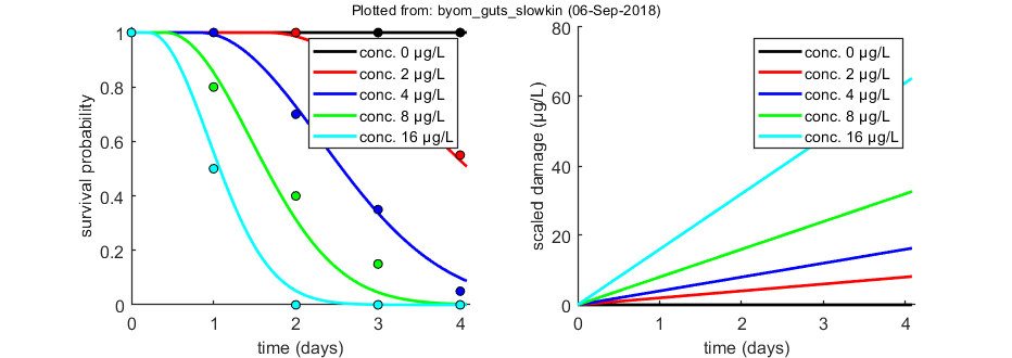
Calculations and plotting
Here, the function is called that will do the calculation and the plotting.
glo.useode = 0; % calculate model using ODE solver (1) or analytical solution (0)
if glo.sel == 1 % for the pure SD model, turn on the events function to catch threshold exceedance
    glo.eventson = 1; % events function on (1) or off (0)
end

opt_optim.fit = 1; % fit the parameters (1), or don't (0)
opt_optim.it  = 0; % show iterations of the optimisation (1, default) or not (0)

glo.fastslow = 's'; % tell simplefun that we need slow (s) or fast (f) kinetics
% slow kinetics implies that mw is now used for mw/kd and bw becomes bw*kd!
% so we need to modify initial values for some parameters:
par.kd(2) = 0; % don't fit the dominant rate constant anymore
par.mw(1) = 0.7; % NOTE: this is now mw/kd!
par.bw(1) = 0.07; % NOTE: this is now bw*kd!

% optimise and plot (fitted parameters in par_out)
par_out = calc_optim(par,opt_optim); % start the optimisation
calc_and_plot(par_out,opt_plot); % calculate model lines and plot them
Goodness-of-fit measures for each data set (R-square)
    0.9912

Warning: R-square is not appropriate for survival data and needs to be
interpreted more qualitatively!

=================================================================================
Results of the parameter estimation with BYOM version 4.2b
=================================================================================
   Filename      : byom_guts_slowkin
   Analysis date : 06-Sep-2018 (16:07)
   Data entered  :
     data state 1: 5x5, survival data.
     data state 2: 0x0, no data.
   Search method: Nelder-Mead simplex direct search, 2 rounds.
     The optimisation routine has converged to a solution
     Total 113 simplex iterations used to optimise.
     Minus log-likelihood has reached the value 89.8336 (AIC=185.667).
=================================================================================
kd           0.06 (fit: 0, initial: 0.06)
mw          3.304 (fit: 1, initial: 0.7)
hb      1.492e-08 (fit: 1, initial: 0.001)
bw          0.115 (fit: 1, initial: 0.07)
Fs              1 (fit: 0, initial:  1)
=================================================================================
Parameters kd, mw and bw are fitted on log-scale.
=================================================================================
Time required: 0.3 secs
Plots result from the optimised parameter values.
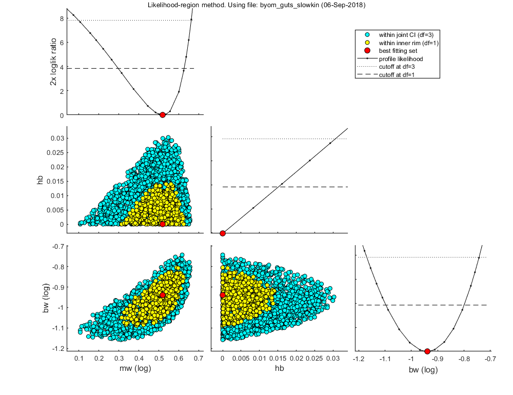
Likelihood region
Make intervals on model predictions by using a sample of parameter sets taken from the joint likelihood-based conf. region.
% UNCOMMENT FOLLOWING LINE(S) TO CALCULATE
opt_likreg.subopt   = 10; % number of sub-optimisations to perform to increase robustness
opt_likreg.detail   = 2; % detailed (1) or a coarse (2) calculation
opt_likreg.burst    = 2000; % number of random sets from parameter space evaluated every iteration
calc_likregion(par_out,500,opt_likreg); % second argument: nr sets in inner region (-1 to re-use saved sample from previous runs)
Calculating profiles and sample from confidence region ... please be patient.

Confidence interval from the profile (single parameter, 95% confidence)
=================================================================================
mw         interval:      1.979 - 4.235
Warning: taking the lowest parameter value as lower confidence limit
hb         interval:          0 - 0.01515
bw         interval:       0.08 - 0.1585

Edges of the joint 95% confidence region (using df=p)
=================================================================================
mw         interval:      1.252 - 4.596
hb         interval:          0 - 0.03063
bw         interval:    0.06766 - 0.1808

  The profiles found a better optimum: 89.8334 (best was 89.8336).
Parameter values for new optimum
=================================================================================
par.kd     = [      0.06  0      0.001         10 0];
par.mw     = [     3.302  1      1e-06      1e+06 0];
par.hb     = [         0  1          0          1 1];
par.bw     = [   0.11444  1      1e-06      1e+06 0];
par.Fs     = [         1  0          1        100 1];
=================================================================================


Starting with obtaining a sample from the joint confidence region.
Bursts of 2000 samples, until at least 500 samples are accepted in inner rim.
Currently accepted (inner rim): 0, 94, 180, 264, 352, 449,

Size of total sample (profile points have been added): 12066
of which accepted in the conf. region: 2247, and in inner rim: 589

Time required: 1 min, 1.0 secs
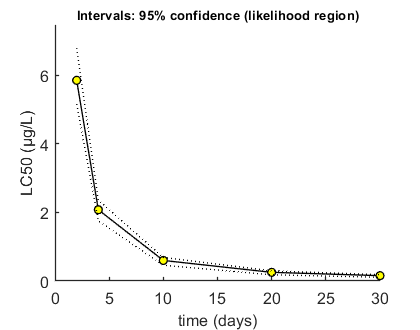
Calculate LCx versus time
Here, the LCx (by default the LC50) is calculated at several time points.
% UNCOMMENT FOLLOWING LINE(S) TO CALCULATE
opt_conf.type    = 2; % use the values from the slice sampler (1) or likelihood region (2) to make intervals
opt_conf.lim_set = 0; % for lik-region sample: use limited set of n_lim points (1) or outer hull (2) to create CIs
opt_lcx.Feff = 0.50; % effect level (>0 en <1), x/100 in LCx

% We can directly use the fast method specific for this reduced GUTS folder
Tend = [2 4 10 20 30]; % times at which to calculate LCx, relative to control
calc_conf_lcx_lim(par_out,Tend,opt_conf,opt_lcx); % calculates LCx values, CI requires that there is a mat file with sample
Calculate LCx values

Amount of 0.4 added to the chi-square criterion for inner rim
  Full sample of 705 sets used.
Calculating CIs on model predictions, using sample from joint likelihood region ... please be patient.

Percentage of sets finished for CIs:   0  10  20  30  40  50  60  70  80  90

Results table for LCx,t (µg/L), with 95% CI
==================================================================
LC50 (   2 days): 5.852 (5.163-6.787)
LC50 (   4 days): 2.077 (1.757-2.361)
LC50 (  10 days): 0.5992 (0.4597-0.6870)
LC50 (  20 days): 0.2525 (0.1811-0.2966)
LC50 (  30 days): 0.1558 (0.1083-0.1858)
==================================================================
Intervals: 95% confidence (likelihood region)

Time required: 1 min, 3.0 secs
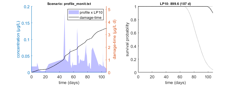
Calculate LPx for a monitoring profile
We can use the function calc_conf_lpx_lim to calculate an exposure multiplication factor: with which factor do we need to multiply an exposure scenario to obtain x% effect at the end of the scenario? Here, done for 10% effect at the end of the exposure scenario.
This is the fast method, which is closely linked to this GUTS model (reduced model, standard directory). Don't use if you modify the GUTS model in simplefun.m, call_deri.m or derivatives.m, unless you know what you are doing.
% UNCOMMENT FOLLOWING LINE(S) TO CALCULATE
opt_conf.type     = 2; % use values from slice sampler (1), likelihood region(2) to make intervals (-1 to skip intervals)
opt_conf.lim_set  = 2; % for lik-region sample: use limited set of n_lim points (1) or outer hull (2) to create CIs
opt_lpx.Feff      = 0.10; % effect level (>0 en <1), x/100 in LCx
glo.useode        = 0; % no need for ODE solver, as long as scen_type = 4 (default, linear forcing)

Tend  = []; % time at which to calculate LPx (empty is end of profile)
LPx_mon = calc_conf_lpx_lim(par_out,Tend,'profile_monit.txt',opt_conf,opt_lpx);
Calculate exposure multiplication factors
==================================================================
LP10 ( 107 days): 899.6
==================================================================

Amount of 0.4 added to the chi-square criterion for inner rim
  Outer hull of 225 sets used.
Calculating CIs on model predictions, using sample from joint likelihood region ... please be patient.

Percentage of sets finished for CIs:   0  10  20  30  40  50  60  70  80  90

Results table for LPx (-) with 95% CI, scenario 1
==================================================================
LP10 ( 107 days): 899.6 (553.1-1134.)
==================================================================
Intervals: 95% confidence (likelihood region)


Amount of 0.4 added to the chi-square criterion for inner rim
  Outer hull of 225 sets used.
Calculating CIs on model predictions, using sample from joint likelihood region ... please be patient.

Percentage of samples finished:    0  10  20  30  40  50  60  70  80  90
Time required: 1 min, 26.8 secs
Time required: 1 min, 26.8 secs