BYOM, byom_doseresp_surv.m

Table of contents

Contents

About

BYOM is a General framework for simulating model systems in terms of ordinary differential equations (ODEs) or explicit functions. This package only supports explicit functions, which are calculated by simplefun.m, which is called by call_deri.m. The files in the BYOM engine directory are needed for fitting and plotting. Results are shown on screen but also saved to a log file (results.out).

The model: Log-logistic dose response fitting.

This script: Example for survival data, using the binomial likelihood function as the error model.

Copyright (c) 2012-2021, Tjalling Jager, all rights reserved.
This source code is licensed under the MIT-style license found in the
LICENSE.txt file in the root directory of BYOM.

Initial things

Make sure that this script is in a directory somewhere below the BYOM folder.

clear, clear global % clear the workspace and globals
global DATA W X0mat % make the data set and initial states global variables
global glo          % allow for global parameters in structure glo
diary off           % turn of the diary function (if it is accidentaly on)
% set(0,'DefaultFigureWindowStyle','docked'); % collect all figure into one window with tab controls
set(0,'DefaultFigureWindowStyle','normal'); % separate figure windows

pathdefine(0) % set path to the BYOM/engine directory (option 1 uses parallel toolbox)
glo.basenm  = mfilename; % remember the filename for THIS file for the plots
glo.saveplt = 0; % save all plots as (1) Matlab figures, (2) JPEG file or (3) PDF (see all_options.txt)

The data set

Data are entered in matrix form, time in rows, scenarios (exposure concentrations) in columns. First column are the exposure times, first row are the concentrations or scenario numbers. The number in the top left of the matrix indicates how to calculate the likelihood:

% Dieldrin survival data for guppies, at t=0 and the end of the test (7
% days). Exposure concentration is in ug/L. More replicates can be entered,
% but only enter one exposure time!
DATA{1} = [-2    7
    0     20
    3.2   18
    5.6   18
    10    8
    18    2
    32    0
    56    0
    100   0 ];

% Weight factors is now the initial number of animals at t=0 in each
% replicate in the data set. Here, all treatments start with the same
% number of animals, so we can define the weights factor with a shortcut.
W{1} = 20*ones(size(DATA{1})-1); % 20 individuals in each treatment

% Derive initial values from the data set, and plotting range for model
% curve. The code below calls a small function with rules-of-thumb to come
% up with relevant starting values.
[Y0,ECx,logc] = startvals(DATA{1},W{1});

Initial values for the state variables

Initial states, scenarios in columns, states in rows. First row are the 'names' of all scenarios.

X0mat(1,:) = DATA{1}(1,2); % assume second element of first row is the scenario (exposure duration)
X0mat(2,:) = 0;  % initial values state 1 (not used)

Initial values for the model parameters

Model parameters are part of a 'structure' for easy reference.

glo.x_EC  = 50; % the x in the ECx
glo.logsc = 1; % plot the dose-response curve on log-scale

% syntax: par.name = [startvalue fit(0/1) minval maxval];
par.ECx  = [ECx  1 0 1e6]; % ECx, with x in glo.x_EC
par.Y0   = [Y0   1 0 1];   % control response (survival probability)
par.beta = [4    1 0 100]; % slope factor of the log-logistic curve

Time vector and labels for plots

Specify what to plot. If time vector glo.t is not specified, a default is used, based on the data set. Note that t is now used for the exposure concentrations!

if glo.logsc == 1 % when plotting on log-scale ...
    % glo.logzero = 0.01; % option to override automatic position for plotting the control treatment on log-scale
    if isfield(glo,'logzero') && log10(glo.logzero) < logc(1) % if we modify the position of the control ...
        logc(1) = log10(glo.logzero) - log10(1.2); % also adapt the lower part of the plotting range
    end
    glo.t = [0,logspace(logc(1),logc(2),300)]; % use a log-spacing for the model curve
    % Note: t=0 needs to be in there for the calculation of the model for the control treatment
else % otherwise ...
    glo.t = linspace(0,10^(logc(2)),300); % otherwise, use a fine linear spacing for the model curve
end

% specify the y-axis labels for each state variable
glo.ylab{1} = 'survival probability';
% specify the x-axis label (same for all states)
glo.xlab    = ['concentration (',char(181),'g/L)'];
glo.leglab1 = 'time '; % legend label before the 'scenario' number
glo.leglab2 = '(d)';   % legend label after the 'scenario' number

prelim_checks % script to perform some preliminary checks and set things up
% Note: prelim_checks also fills all the options (opt_...) with defauls, so
% modify options after this call, if needed.

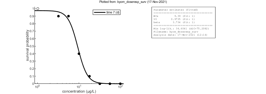
Calculations and plotting

Here, the functions are called that will do the calculation and the plotting. Profile likelihoods are used to make robust confidence intervals. Note that the dose-response curve is plotted on a log scale for the exposure concentration. If the control is truly zero, it is plotted as an open symbol, at a low concentration on the x-axis. However, for the fitting, it is truly zero.

opt_optim.fit  = 1; % fit the parameters (1), or don't (0)
opt_optim.it   = 0; % show iterations of the optimisation (1, default) or not (0)
opt_plot.annot = 1; % extra subplot in multiplot for fits: 1) box with parameter estimates, 2) overall legend

% optimise and plot (fitted parameters in par_out)
par_out = calc_optim(par,opt_optim); % start the optimisation
calc_and_plot(par_out,opt_plot); % calculate model lines and plot them
disp(['x in ECx is: ',num2str(glo.x_EC)])

Goodness-of-fit measures for each state and each data set (R-square)
Based on the individual replicates, accounting for transformations, and including t=0
state 1.   0.99
Warning: R-square is not appropriate for survival data so interpret
qualitatively! 
Warning: (R-square not calculated when missing/removed animals; use plot_tktd) 
 
=================================================================================
Results of the parameter estimation with BYOM version 6.0 BETA 6
=================================================================================
   Filename      : byom_doseresp_surv 
   Analysis date : 17-Nov-2021 (12:14) 
   Data entered  :
     data state 1: 8x1, survival data (dose-response).
   Search method: Nelder-Mead simplex direct search, 2 rounds. 
     The optimisation routine has converged to a solution
     Total 107 simplex iterations used to optimise. 
     Minus log-likelihood has reached the value 34.60 (AIC=75.21). 
=================================================================================
ECx         9.390 (fit: 1, initial: 7.483) 
Y0         0.9735 (fit: 1, initial:  1) 
beta        3.734 (fit: 1, initial:  4) 
=================================================================================
Time required: 0.1 secs
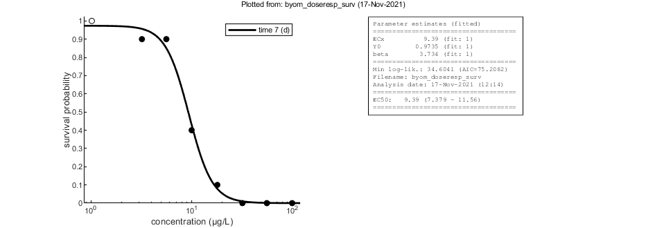
Plots result from the optimised parameter values. 

Due to your small screen size, all multiplots 2x2 and larger will be scaled down.

x in ECx is: 50

Profiling the likelihood

By profiling you make robust confidence intervals for one or more of your parameters. Use the names of the parameters as they occurs in your parameter structure par above. This can be a single string (e.g., 'ECx'), a cell array of strings (e.g., {'ECx','beta'}), or 'all' to profile all fitted parameters. This example produces a profile for ECx and provides the 95% confidence interval (on screen and indicated by the horizontal broken line in the plot).

Options for profiling can be set using opt_prof (see prelim_checks.m).

Note: in this example, the CI for the control response (Y0) runs into its upper boundary of 1 (which is no problem, as it implies 100% survival in the control).

[par_better,Xing] = calc_proflik(par_out,'ECx',opt_prof,opt_optim); % calculate a profile
% Note that the confidence intervals our now returned in _Xing_ (as
% crossings of the chi-square criterion), which contains the CIs for all
% profiled parameters as a cell array. Below, the CI for ECx (in _Xing{1}_)
% is added to the annotation box for subsequent plotting.
glo.str_extra{1} = sprintf('EC%1.0f: %6.4g (%4.4g - %4.4g)',glo.x_EC, par_out.ECx(1),Xing{1}([1 end],1));
calc_and_plot(par_out,opt_plot); % calculate model lines and plot them

  
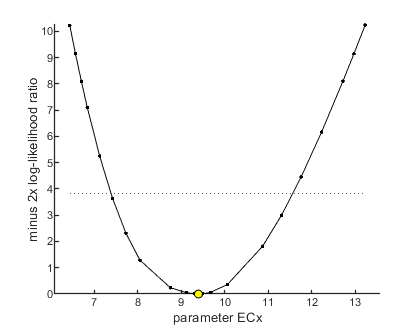
95% confidence interval(s) from the profile(s)
=================================================================================
ECx        interval:      7.379 -  11.56 
=================================================================================
 
Time required: 2.2 secs
Plots result from the optimised parameter values. 

Due to your small screen size, all multiplots 2x2 and larger will be scaled down.

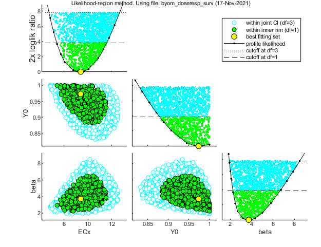
Likelihood region

Another way to make intervals on model predictions is to use a sample of parameter sets taken from the joint likelihood-based conf. region. This is done by the function calc_likregion.m. It first does profiling of all fitted parameters to find the edges of the region. Then, Latin-Hypercube sampling, keeping only those parameter combinations that are not rejected at the 95% level in a lik.-rat. test. The inner rim will be used for CIs on forward predictions.

Options for the likelihood region can be set using opt_likreg (see prelim_checks.m). For the profiling part, use the options in opt_prof.

% UNCOMMENT LINE(S) TO CALCULATE
opt_likreg.detail   = 2; % detailed (1) or a coarse (2) calculation
opt_likreg.subopt   = 0; % number of sub-optimisations to perform to increase robustness
opt_likreg.burst    = 1000; % number of random samples from parameter space taken every iteration
calc_likregion(par_out,500,opt_likreg,opt_prof,opt_optim);
% Second entry is the number of accepted parameter sets to aim for. Use -1
% here to use a saved set.

 
Calculating profiles and sample from confidence region ... please be patient.
  
95% confidence interval(s) from the profile(s)
=================================================================================
ECx        interval:      7.379 -  11.56 
Y0         interval:     0.8790 - >1.000 
beta       interval:      2.255 -  6.663 
=================================================================================
 
Time required: 4.2 secs
 
Starting with obtaining a sample from the joint confidence region.
Bursts of 1000 samples, until at least 500 samples are accepted in inner rim.
Total number of parameters tried (profile points have been added): 6050
of which accepted in the conf. region: 1811, and in inner rim: 624

 
Time required: 6.1 secs

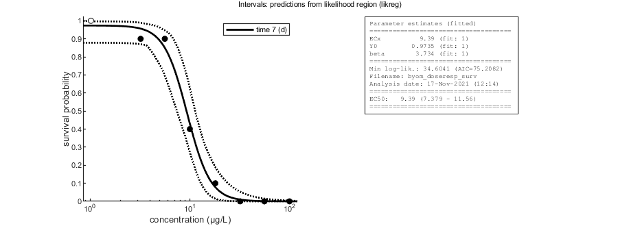
Plot results with confidence intervals

The following code can be used to make a standard plot (the same as for the fits), but with confidence intervals. Options for confidence bounds on model curves can be set using opt_conf (see prelim_checks).

Use opt_conf.type to tell calc_conf which sample to use: -1) Skips CIs (zero does the same, and an empty opt_conf as well). 1) Bayesian MCMC sample (default); CI on predictions are 95% ranges on the model curves from the sample 2) parameter sets from a joint likelihood region using the shooting method (limited sets can be used), which will yield (asymptotically) 95% CIs on predictions 3) as option 2, but using the parameter-space explorer

% UNCOMMENT LINE(S) TO CALCULATE
opt_conf.type    = 2; % use the values from the slice sampler (1) or likelihood region (2) to make intervals
opt_conf.lim_set = 2; % use limited set of n_lim points (1) or outer hull (2, likelihood methods only) to create CIs

out_conf = calc_conf(par_out,opt_conf); % calculate confidence intervals on model curves
calc_and_plot(par_out,opt_plot,out_conf); % call the plotting routine again to plot fits with CIs

 
Amount of 0.3764 added to the chi-square criterion for inner rim
Slightly more is taken to provide a generally conservative estimate of the CIs.
  Outer hull of 269 sets used.
Calculating CIs on model predictions, using sample from joint likelihood region ... please be patient.
 
Time required: 6.5 secs
Plots result from the optimised parameter values. 

Due to your small screen size, all multiplots 2x2 and larger will be scaled down.

Published with MATLAB® R2021b