Entering data into BYOM
Back to the overview of the manual
Contents
BYOM offers a lot of flexibility in entering all sorts of data, in all kinds of formats. In this section, I will try to present all of the possible ways to enter data ...
lets_get_started
Basic data sets
We already seen the most basic option to enter data in the getting started section. Let's take a very simple and short example with three time points and two scenarios:
DATA{1} = [1  0.1 0.2
           0    0   0
           1    2   4
           2    3   7];
If these observations are means, it is generally a good idea to provide the weight factors as the number of individuals on which a mean is based. Note that this will not always lead to a different fit, and that for survival data (using a -1 in the top-left corner of the data matrix) the weight matrix is used differently. Suppose we have two replicates for each observation, we can enter a weight matrix as follows:
W{1} = [2 2
        2 2
        2 2];
The weight matrix has a {1} to signify that it belongs to state variable 1, just like DATA{1}, and has the same size as DATA{1} without the concentration and time vectors (feel free to include them, but they will be ignore anyway). If a weight matrix is not provided, ones will be used (and zeros for survival data).
If we have values for the two replicates at each time point, it is a good idea to use them instead of the mean. There are two basic ways to enter replicates. The first is to duplicate the scenarios:
DATA{1} = [1  0.1 0.1 0.2 0.2
           0    0   0   0   0
           1    1   3   3   5
           2    2   4   5   9];
However, we can also duplicate time points, with the same effect:
 DATA{1} = [1  0.1 0.2
           0    0   0
           0    0   0
           1    1   3
           1    3   5
           2    2   5
           2    4   9];
Even though both version will yield the same fit, the first one is preferred: several plotting routines have the possibility to plot means with CIs or individual replicates. However, the latter data definition can only be plotted as individual replicates.
Matlab requires matrices to be square. If you have a missing value somewhere, make sure you enter a NaN (Matlabs for 'not a number').
Combining data sets
Suppose we have the data in a format as two separate sets:
  D_1 = [1  0.1
         0    0
         1    2
         2    3];

  D_2 = [1  0.2
         0    0
         1    4
         2    7];
No need to do reformatting by hand or in Excel (and possibly introduce errors). We can easily combine both sets within BYOM by using the function mat_combine:
DATA{1} = mat_combine(0,D_1,D_2); % combine two data matrices

DATA{1} % display the results on screen to see what happened
ans =

    1.0000    0.1000    0.2000
         0         0         0
    1.0000    2.0000    4.0000
    2.0000    3.0000    7.0000
The 0 in the call to mat_combine is to tell the function to replace missing points with a NaN (use a 1 to estimate them by interpolation). We can illustrate this by using two data sets with a different time vector:
  D_1 = [1  0.1
         0    0
         1    2
         2    3];

  D_2 = [1  0.2
         0    0
         0.5  4
         3    7];

DATA{1} = mat_combine(0,D_1,D_2); % combine two data matrices

DATA{1} % display the results on screen to see what happened
ans =

    1.0000    0.1000    0.2000
         0         0         0
    0.5000       NaN    4.0000
    1.0000    2.0000       NaN
    2.0000    3.0000       NaN
    3.0000       NaN    7.0000
This function does not care when there the scenarios overlap between two data sets (they are simply duplicated into the result). However, do not use mat_combine when there are duplicates in the time vector of one the sets (you will get an error message). In any case, it never hurts to check whether this function acted as expected by checking the data matrix that comes out. This function can also be called with more than two data sets.
Another way to include multiple data sets for the same state is to define them as additional data sets for the same state variable 1. For example:
  DATA{1,1} = [1  0.1
         0    0
         1    2
         2    3];

  DATA{2,1} = [1  0.2
         0    0
         0.5  4
         3    7];
Defining multiple data sets like this needs to be carefully considered. Firstly, it may be confusing if you have multiple states as well. For example, if you have two states, you should define DATA{1,2} and DATA{2,2} as well, which can be confusing. Furthermore, the results for both data sets will be plotted in separate figure windows. And, finally, the statistical treatment is different when using multiple data sets or when combining them into one. Within a data set, all data points (if needed, after transformation) are assumed to have the same residual variance. If we define two data sets, these residual variances may differ (which may be what we want, or not). The function transfer contains an option to force the same residual variance on multiple data sets.
Data that don't match state vs. time
The way of specifying data sets in BYOM assumes that there is an independent variable (generally 'time') against which the observations on a state variable can be plotted. Some types of data, however, do not fall neatly into this category.
Zero-variate data. Suppose I have an energy-budget model that specifies growth and reproduction of an animal. I have data on length versus time (which can go into DATA{1}), but for reproduction I only have a maximum reproduction rate of 120 eggs/day (something that I cannot put a time point on, and cannot go nicely into DATA{2}). The model parameters that I want to fit do specify the maximum reproduction rate, but to include this 'zero-variate' information into the fit, we need to enter them differently:
zvd.Rm = [120 5]; % zero-variate data point with normal s.d.
Note that I have to specify a standard deviation to judge the residual (the difference between the model prediction and the single data point). As there is only a single data point, there is no information in the data set itself on the residual variance. I assume that a normal distribution is appropriate. Somewhere, we need to tell the fitting routine what model prediction to compare this zero-variate data point to. This needs to be done in call_deri. For example, if the maximum reproduction rate is the product of parameter a and b:
zvd.Rm(3) = par.a(1) * par.b(1); % predicted max. repro rate
The model estimate is thus added to zvd.Rm at the third position of the vector. You can use as many zero-variate data points as you like, and name them any way you like. They only exist within the global zvd structure. The zero-variate data points and their model estimate will be plotted in a separate figure window. An example is provided in the 'extra' example of BYOM.
Output mapping. Sometimes are data are in a different format than the state variables of the model. For example, the state variable of the model is body length and your data are in body weight, or your data represent the sum of two state variables. BYOM includes a simple way to map state variables onto data sets (by default, state variable i is mapped onto data set i).
This is done in call_deri that contains a specific section for that purpose. The matrix Xout contains a row for each state variable. Here, you can transform any of the columns to match the data, or sum two columns to make a new one, etc. The Xout will be compared to the data in DATA. Column 1 of Xout is compared to DATA{1}, for each treatment. Note that in call_deri, the scenarios enter one at a time.
The 'extra' data set. In some cases, output mapping does not help, for example becuase are states are functions of time but our data are not. For example, suppose we have an energy-budget model with the state variable body size and reproduction. We may have data for these endpoints over time, but we also have data for ingestion rate as a function of body size. The latter type of data cannot be entered in the DATA array, which always links to the state variables over time.
For such situations, we can define an extra data set as, for example:
DATAx{1} = [1      0.1    0.2
            0.257 0.75    NaN
            0.223  NaN  0.697
            0.467 1.24    NaN
            0.398  NaN   1.14];
In this example, we have two scenarios (0.1 and 0.2), the data are not transformed (the 1 in the top-left corner), and we have observations of ingestion at several body sizes (first column). The tricky part is now to reprogramme call_deri to obtain matching model values for these observations! For this reason, an additional output matrix Xout2 can be used, which needs to match the data set. Unlike observation at a given time, we cannot now calculate model values at the exact location of the observation (in our example, the x-axis of the extra data is body size, a state variable of the model). In transfer, the values in Xout2 will be interpolated to match the x-values in the extra data set. The format of Xout2 is different from the standard Xout: it is an array rather than a matrix. So, we need to specify Xout2{1} to be compared to DATAx{1}. The extra data sets, and the corresponding model prediction, will be plotted in a separate figure. You can specify axis labels for this figure in the main script using xlab2{1} and ylab2{1}.
I realise that this requires far more explanation before you can actually use this yourself. I will try to make an example for this type of use of BYOM. However, it is good to know that this option exists, and that there is no simpler solution for this type of data sets.
Time-varying forcings
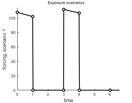
Sometimes, a data set is used as a forcing function for the model, and not as something to fit on. A good example is the use of measured (or estimated) exposure concentrations in a pulse-exposure toxicity experiment. The function derivatives needs to have a concentration at each possible value for time t, but we have measurements only at a few times. The solution is to interpolate in the exposure values. We don t use the global array DATA in this case for the exposure concentrations, as we are going to work with this data set as a forcing function and not as observations on a state variable. For example, we have an exposure scenario with two pulses for the water concentration Cw:
Cw = [0   1
    0   108
    1   102
    1.01  0
    2.99  0
    3   112
    4   107
    4.01  0
    6     0];
Note that we still need to have a scenario number in the first row, as we might have different forcing functions for each treatment. You need to use this identifier in DATA and in X0mat, and it will enter in derivatives as the variable c. The number in the top-left corner is now ignored; these data are not fitted but interpolated. We can prepare this data set for splining with the following utility:
make_scen(4,Cw); % prepare as linear-forcing function interpolation
This function prepares Cw to act as an exposure scenarion, makes a plot so you can inspect the result, and places the scenario information into the global glo for derivatives to use. The 4 is used for linear interpolation, but other options, such as instantaneous pulses, are available.
Next, we have to tell derivatives how to use it. In derivatives add the following code, after the definition of the globals (so glo is known), and before using the concentration Cw in the ODE:
Cw = read_scen(-1,c,t,glo); % use read_scen to derive actual exposure concentration at time t
The result is that scenario Cw is now the concentration at time t as interpolated from the spline for this scenario. Please note that this will make your analysis slower: the exposure concentration now changes rapidly in time, which the ODE solver does not like. You can try different solvers to see if that speeds things up. Several of the packages for GUTS and DEBtox have elegant solutions for this.
Extras
Weighing each data set differently. In some cases, it may be necessary to weigh complete data sets differently. For example, I have two state variables, and I want to make sure that the model fits state 1 as closely as possible, at the expense of the fit to state 2. Below the parameter definition, set this global option:
glo.wts = [10 1]; % extra weight factor for each data set
This gives the data for state 1 twice the weight as that of state 2. If we included two data sets for one state, we need to specify the weights as:
glo.wts = [10;1]; % extra weight factor for each data set
In that case, the first data set for state 1 gets 10 times the weight of the second data set for state 1. If you use this option, make sure that the matrix entered in glo.wts has exactly the same size as the data set (try: size(DATA) at the Matlab prompt when in doubt).
Residual variance for each data set. By default, the residual variance is derived from the data themselves, automatically (see the technical document on http://www.debtox.info/book.html on treating the s.d. as a 'nuisance parameter'). This generally works very well. However, for very small data sets this might produce unwanted results, especially when the model can go exactly through the data point(s). In those cases, it makes sense to specify the residual variance for each data set using an additional global option. For an example with two state variables:
glo.var = [0.12 0.41]; % supply residual variance for two states
If you apply transformations, this is the variance after transformation. As with the glo.wts above, the glo.var must have the same size as the data set. For survival data, the entry in glo.var is meaningless, and is ignored. If your data are means, and only the variance of the mean is known, enter that variance times the number of replicates.