BYOM, byom_my_first.m, a quick example
This script is a full working example of a BYOM analysis, published with the Matlab 'publish' option. The model equations are included in the function derivatives.m.
- Author: Tjalling Jager
- Date: November 2021
- Web support: http://www.debtox.info/byom.html
- Back to getting started or main index
BYOM is a General framework for simulating model systems in terms of ordinary differential equations (ODEs). The model itself needs to be specified in derivatives.m, and call_deri.m may need to be modified to the particular problem as well. The files in the engine directory are needed for fitting and plotting. Results are shown on screen but also saved to a log file (results.out).
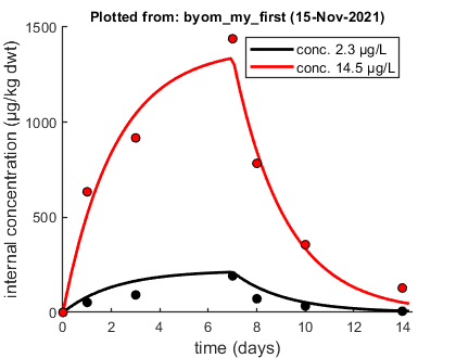
The model: An organism is exposed to a chemical in its surrounding medium. The animal accumulates the chemical according to standard one-compartment first-order kinetics, specified by an uptake rate constant (ku) and an elimination rate (ke).
This script: Data from Gomez et al. (2012), http://dx.doi.org/10.1007/s11356-012-0964-3 on accumulation of tetrazepam in Mytilus galloprovincialis. This set of files is a slight modification from the basic example file for the BYOM platform.
Copyright (c) 2012-2021, Tjalling Jager, all rights reserved.
This source code is licensed under the MIT-style license found in the
LICENSE.txt file in the root directory of BYOM.
Contents
Initial things
Make sure that this script is in a directory somewhere below the BYOM folder. First, some globals are defined, and some housekeeping is done.
clear, clear global % clear the workspace and globals
global DATA W X0mat % make the data set and initial states global variables
global glo          % allow for global parameters in structure glo
diary off           % turn of the diary function (if it is accidentaly on)
% set(0,'DefaultFigureWindowStyle','docked'); % collect all figure into one window with tab controls
set(0,'DefaultFigureWindowStyle','normal'); % separate figure windows

pathdefine % set path to the BYOM/engine directory automatically
glo.basenm  = mfilename; % remember the filename for THIS file for the plots
The data set
Data are entered in matrix form, time in rows, scenarios (exposure concentrations) in columns. First column are the exposure times, first row are the concentrations or scenario numbers. The number in the top left of the matrix indicates how to calculate the likelihood:
- -1 for multinomial likelihood (for survival data)
- 0 for log-transform the data, then normal likelihood
- 0.5 for square-root transform the data, then normal likelihood
- 1 for no transformation of the data, then normal likelihood
% Internal concentration in mussels in ug/kg dwt, time in days, exposure
% concentrations in ug/L.
DATA{1} = [1           2.3         14.5
            0            0            0
            1       52.542        634.1
            3       92.128       917.68
            7       192.17       1438.8
            8       71.975       783.81
           10       33.108       356.28
           14       6.4778       128.48];

% If weight factors are not specified, ones are used.
Initial values for the state variables
Initial states, scenarios in columns, states in rows. First row are the 'names' of all scenarios.
X0mat = [2.3 14.5  % the scenarios (here exposure concentrations)
         0   0  ];  % initial values state 1 (internal concentrations)
Initial values for the model parameters
Model parameters are part of a 'structure' for easy reference.
% syntax: par.name = [startvalue fit(0/1) minval maxval];
par.Kiw   = [50  1    0 1e6];   % bioconcentration factor, L/kg
par.ke    = [0.2 1 1e-3 100];  % elimination rate constant, d-1
Time vector and labels for plots
Specify what to plot. If time vector glo.t is not specified, a default is used, based on the data set
% specify the y-axis labels for each state variable
glo.ylab{1} = ['internal concentration (',char(181),'g/kg dwt)'];
% specify the x-axis label (same for all states)
glo.xlab    = 'time (days)';
glo.leglab1 = 'conc. '; % legend label before the 'scenario' number
glo.leglab2 = [char(181),'g/L'];   % legend label after the 'scenario' number

prelim_checks % script to perform some preliminary checks and set things up
% Note: prelim_checks also fills all the options (opt_...) with defaults,
% so modify options after this call, if needed.
Calculations and plotting
Here, the functions are called that will do the calculation and the plotting.
opt_optim.fit = 1; % fit the parameters (1), or don't (0)
opt_optim.it  = 0; % show iterations of the optimisation (1, default) or not (0)

% optimise and plot (fitted parameters in par_out)
par_out = calc_optim(par,opt_optim); % start the optimisation
calc_and_plot(par_out,opt_plot); % calculate model lines and plot them
Goodness-of-fit measures for each state and each data set (R-square)
Based on the individual replicates, accounting for transformations, and including t=0
state 1.   0.98
=================================================================================
Results of the parameter estimation with BYOM version 6.0 BETA 6
=================================================================================
   Filename      : byom_my_first
   Analysis date : 15-Nov-2021 (16:43)
   Data entered  :
     data state 1: 7x2, continuous data, no transf.
   Search method: Nelder-Mead simplex direct search, 2 rounds.
     The optimisation routine has converged to a solution
     Total 69 simplex iterations used to optimise.
     Minus log-likelihood has reached the value 84.13 (AIC=172.26).
=================================================================================
Kiw         95.99 (fit: 1, initial: 50)
ke         0.4625 (fit: 1, initial: 0.2)
=================================================================================
Time required: 0.5 secs
Plots result from the optimised parameter values.
Profiling the likelihood
By profiling you make robust confidence intervals for one or more of your parameters. Use the name of the parameter as it occurs in your parameter structure par above. This can be a single string (e.g., 'r'), a cell array of strings (e.g., {'r','K'}), or 'all' to profile all fitted parameters.
% run a profile for selected parameters ...
calc_proflik(par_out,'all',opt_prof);  % calculate a profile for all fitted parameters
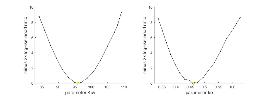
95% confidence interval(s) from the profile(s)
=================================================================================
Kiw        interval:      88.86 -  103.8
ke         interval:     0.3805 -  0.5516
=================================================================================

Time required: 5.9 secs