BYOM, byom_doseresp_propazo.m

Table of contents

About
Initial things
The data set
Initial values for the state variables
Initial values for the model parameters
Time vector and labels for plots
Calculations and plotting
Other files: simplefun

About

Author: Tjalling Jager
Date: November 2021
Web support: http://www.debtox.info/byom.html
Back to index walkthrough_doseresp.html

BYOM is a General framework for simulating model systems in terms of ordinary differential equations (ODEs) or explicit functions. This package only supports explicit functions, which are calculated by simplefun.m, which is called by call_deri.m. The files in the BYOM engine directory are needed for fitting and plotting. Results are shown on screen but also saved to a log file (results.out).

The model: Log-logistic dose response fitting.

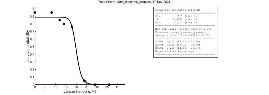
This script: Example for survival data, using the binomial likelihood function as the error model. Data for propiconazole in Gammarus pulex from Nyman et al, 2012 (DOI 10.1007/s10646-012-0917-0). This script demonstrates how to calculate and plot ECx for a range of x-values, and how to plot all ECx values with their CIs into the annotation box in the plot.

Copyright (c) 2012-2021, Tjalling Jager, all rights reserved.
This source code is licensed under the MIT-style license found in the
LICENSE.txt file in the root directory of BYOM.

Initial things

Make sure that this script is in a directory somewhere below the BYOM folder.

clear, clear global % clear the workspace and globals
global DATA W X0mat % make the data set and initial states global variables
global glo          % allow for global parameters in structure glo
diary off           % turn of the diary function (if it is accidentaly on)
% set(0,'DefaultFigureWindowStyle','docked'); % collect all figure into one window with tab controls
set(0,'DefaultFigureWindowStyle','normal'); % separate figure windows

pathdefine(0) % set path to the BYOM/engine directory (option 1 uses parallel toolbox)
glo.basenm  = mfilename; % remember the filename for THIS file for the plots
glo.saveplt = 0; % save all plots as (1) Matlab figures, (2) JPEG file or (3) PDF (see all_options.txt)

The data set

Data are entered in matrix form, time in rows, scenarios (exposure concentrations) in columns. First column are the exposure times, first row are the concentrations or scenario numbers. The number in the top left of the matrix indicates how to calculate the likelihood:

-2 for binomial likelihood (dose-response fitting of survival data)
-1 for multinomial likelihood (for survival data)
0 for log-transform the data, then normal likelihood
0.5 for square-root transform the data, then normal likelihood
1 for no transformation of the data, then normal likelihood

% Full data set with observed number of survivors, time in days, conc in uM
% Note: this is the matrix format used for GUTS analysis.
D = [-2	0	8.1	12	14	18	24	29	36
    0	20	20	20	20	21	20	20	20
    1	19	20	19	19	21	17	11	11
    2	19	20	19	19	20	6	4	1
    3	19	20	19	18	16	2	0	0
    4	19	19	17	16	16	1	0	0];

% Select one time point from the data set for dose-response analysis. More
% replicates can be entered, but only enter one exposure time!
T = 4; % e.g., 4 days (end of experiment)
ind_T = find(D(2:end,1)==T); % index to the requested time point
DATA{1} = [D(1,:)' D(ind_T+1,:)']; % select concentrations and survivors and put them into columns

% Weight factors is now the initial number of animals at t=0 in each
% replicate in the data set.
W{1} = D(2,2:end)'; % copy row at t=0 and turn it into a column
% There are 20 or 21 individuals in each treatment; here we take the first
% row of survivor data from the dataset D above, and turn it into a column
% vector.

% Derive initial values from the data set, and plotting range for model
% curve. The code below calls a small function with rules-of-thumb to come
% up with relevant starting values.
[Y0,ECx,logc] = startvals(DATA{1},W{1});

Initial values for the state variables

Initial states, scenarios in columns, states in rows. First row are the 'names' of all scenarios.

X0mat(1,:) = DATA{1}(1,2); % take second element of first row is the scenario (exposure duration)
X0mat(2,:) = 0;  % initial values state 1 (not used)

Initial values for the model parameters

Model parameters are part of a 'structure' for easy reference.

glo.logsc = 0; % plot the dose-response curve on log-scale

% syntax: par.name = [startvalue fit(0/1) minval maxval];
par.ECx  = [ECx  1 0 1e6]; % ECx, with x in glo.x_EC
par.Y0   = [Y0   1 0 1];   % control response (survival probability)
par.beta = [4    1 0 100]; % slope factor of the log-logistic curve

Time vector and labels for plots

Specify what to plot. If time vector glo.t is not specified, a default is used, based on the data set. Note that t is now used for the exposure concentrations!

if glo.logsc == 1 % when plotting on log-scale ...
    % glo.logzero = 0.01; % option to override automatic position for plotting the control treatment on log-scale
    if isfield(glo,'logzero') && log10(glo.logzero) < logc(1) % if we modify the position of the control ...
        logc(1) = log10(glo.logzero) - log10(1.2); % also adapt the lower part of the plotting range
    end
    glo.t = [0,logspace(logc(1),logc(2),300)]; % use a log-spacing for the model curve
    % Note: t=0 needs to be in there for the calculation of the model for the control treatment
else % otherwise ...
    glo.t = linspace(0,10^(logc(2)),300); % otherwise, use a fine linear spacing for the model curve
end

% specify the y-axis labels for each state variable
glo.ylab{1} = 'survival probability';
% specify the x-axis label (same for all states)
glo.xlab    = ['concentration (',char(181),'M)'];
glo.leglab1 = 'time '; % legend label before the 'scenario' number
glo.leglab2 = '(d)';   % legend label after the 'scenario' number

prelim_checks % script to perform some preliminary checks and set things up
% Note: prelim_checks also fills all the options (opt_...) with defauls, so
% modify options after this call, if needed.

Calculations and plotting

Here, the functions are called that will do the calculation and the plotting. Profile likelihoods are used to make robust confidence intervals. Note that the dose-response curve is plotted on a log scale for the exposure concentration. If the control is truly zero, it is plotted as an open symbol, at a low concentration on the x-axis. However, for the fitting, it is truly zero.

opt_optim.fit   = 1; % fit the parameters (1), or don't (0)
opt_optim.it    = 0; % show iterations of the optimisation (1, default) or not (0)
opt_plot.annot  = 1; % extra subplot in multiplot for fits: 1) box with parameter estimates, 2) overall legend
opt_plot.legsup = 1; % set to 1 to suppress legends on fits

% Optimisation and profiling is done three times to obtain EC50, EC20 and
% EC10 with their confidence intervals. An initial value for ECx is
% estimated from the data set by interpolation (this might not work for all
% data sets, so you may need to provide manual starting values when the fit
% looks poor and/or profiling finds a better optimum). The results are
% collected in a string that is passed to calc_and_plot in the global glo
% for annotation.

x_EC = [50 20 10]; % values for x in ECx to run through

str_ecx = cell(1,length(x_EC));
for i = 1:length(x_EC) % run through all x values
    glo.x_EC  = x_EC(i); % the x in the ECx; put in global variable glo
    % Do optimisation
   [par_out,mll(i)] = calc_optim(par,opt_optim); % start the optimisation
    disp(['x in ECx is: ',num2str(glo.x_EC)]) % output current effect percentage to screen
    % Calculate confidence intervals by profiling the likelihood
    [par_better,Xing] = calc_proflik(par_out,'ECx',opt_prof,opt_optim); % calculate a profile
    % Create text line to go into the figure window, using the output from
    % the fitting (the best fit) and the profiling (the confidence interval).
    str_ecx{i} = sprintf('EC%1.0f: %#6.4g (%#4.4g - %#4.4g)',glo.x_EC, par_out.ECx(1),Xing{1}([1 end],1));
end

if max(abs(diff(mll))) > 1e-6
    error('The minus log-likelihood of the fits seem to differ between the runs; check your results.')
end

% Add a line to the annotation box in the plot to clarify the likelihood
% function that was used
switch DATA{1}(1)
    case -2
        str_ecx{end+1} = ['Binomial likelihood used'];
    case -1
        error('The multinomial likelihood cannot be used for dose-response data in this package');
    case 1
        str_ecx{end+1} = ['Normal likelihood used'];
    case 0
        str_ecx{end+1} = ['Normal likelihood used (log transformed)'];
    case 0.5
        str_ecx{end+1} = ['Normal likelihood used (sqrt transformed)'];
    otherwise
        str_ecx{end+1} = ['Normal likelihood used (power ',num2str(DATA{1}(1)),' transformed)'];
end

glo.str_extra = str_ecx; % place the collected strings into the global
calc_and_plot(par_out,opt_plot); % calculate model lines and plot them
% Note: the plot is for the last fit, but they should be all the same

Goodness-of-fit measures for each state and each data set (R-square)
Based on the individual replicates, accounting for transformations, and including t=0
state 1.   0.99
Warning: R-square is not appropriate for survival data so interpret
qualitatively! 
Warning: (R-square not calculated when missing/removed animals; use plot_tktd) 
 
=================================================================================
Results of the parameter estimation with BYOM version 6.0 BETA 6
=================================================================================
   Filename      : byom_doseresp_propazo 
   Analysis date : 17-Nov-2021 (12:15) 
   Data entered  :
     data state 1: 8x1, survival data (dose-response).
   Search method: Nelder-Mead simplex direct search, 2 rounds. 
     The optimisation routine has converged to a solution
     Total 113 simplex iterations used to optimise. 
     Minus log-likelihood has reached the value 43.64 (AIC=93.27). 
=================================================================================
ECx         20.07 (fit: 1, initial: 20.78) 
Y0         0.8893 (fit: 1, initial: 0.95) 
beta        16.03 (fit: 1, initial:  4) 
=================================================================================
Time required: 0.2 secs
x in ECx is: 50

  
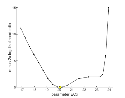
95% confidence interval(s) from the profile(s)
=================================================================================
ECx        interval:      18.55 -  23.58 
=================================================================================
 
Time required: 1.1 secs
Goodness-of-fit measures for each state and each data set (R-square)
Based on the individual replicates, accounting for transformations, and including t=0
state 1.   0.99
Warning: R-square is not appropriate for survival data so interpret
qualitatively! 
Warning: (R-square not calculated when missing/removed animals; use plot_tktd) 
 
=================================================================================
Results of the parameter estimation with BYOM version 6.0 BETA 6
=================================================================================
   Filename      : byom_doseresp_propazo 
   Analysis date : 17-Nov-2021 (12:15) 
   Data entered  :
     data state 1: 8x1, survival data (dose-response).
   Search method: Nelder-Mead simplex direct search, 2 rounds. 
     The optimisation routine has converged to a solution
     Total 119 simplex iterations used to optimise. 
     Minus log-likelihood has reached the value 43.64 (AIC=93.27). 
=================================================================================
ECx         18.41 (fit: 1, initial: 20.78) 
Y0         0.8893 (fit: 1, initial: 0.95) 
beta        16.03 (fit: 1, initial:  4) 
=================================================================================
Time required: 1.1 secs
x in ECx is: 20

  
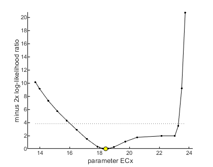
95% confidence interval(s) from the profile(s)
=================================================================================
ECx        interval:      16.02 -  23.29 
=================================================================================
 
Time required: 2.2 secs
Goodness-of-fit measures for each state and each data set (R-square)
Based on the individual replicates, accounting for transformations, and including t=0
state 1.   0.99
Warning: R-square is not appropriate for survival data so interpret
qualitatively! 
Warning: (R-square not calculated when missing/removed animals; use plot_tktd) 
 
=================================================================================
Results of the parameter estimation with BYOM version 6.0 BETA 6
=================================================================================
   Filename      : byom_doseresp_propazo 
   Analysis date : 17-Nov-2021 (12:15) 
   Data entered  :
     data state 1: 8x1, survival data (dose-response).
   Search method: Nelder-Mead simplex direct search, 2 rounds. 
     The optimisation routine has converged to a solution
     Total 133 simplex iterations used to optimise. 
     Minus log-likelihood has reached the value 43.64 (AIC=93.27). 
=================================================================================
ECx         17.50 (fit: 1, initial: 20.78) 
Y0         0.8893 (fit: 1, initial: 0.95) 
beta        16.03 (fit: 1, initial:  4) 
=================================================================================
Time required: 2.2 secs
x in ECx is: 10

  
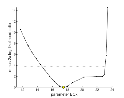
95% confidence interval(s) from the profile(s)
=================================================================================
ECx        interval:      14.59 -  23.07 
=================================================================================
 
Time required: 3.1 secs
Plots result from the optimised parameter values. 

Due to your small screen size, all multiplots 2x2 and larger will be scaled down.

Other files: simplefun

To archive analyses, publishing them with Matlab is convenient. To keep track of what was done, the file simplefun.m can be included in the published result. This includes the actual model equation.

%% BYOM function simplefun.m (the model as explicit equations)
%
%  Syntax: Xout = simplefun(t,X0,par,c,glo)
%
% This function calculates the output of the model system. It is linked to
% the script files named byom_doseresp_*.m. Therefore, _t_ is used for
% concentrations and _c_ for time! (Note: BYOM normally works with 'time'
% on the x-axis). As input, it gets:
%
% * _t_   is the vector with exposure concentrations
% * _X0_  is a vector with the initial values for states (not used)
% * _par_ is the parameter structure
% * _c_   is the exposure time at which the dose-response is made
% * _glo_ is the structure with information (normally global)
%
% Variable _t_ is handed over as a vector, and scenario name _c_ as single
% number, by <call_deri.html call_deri.m> (you do not have to use them in
% this function). Output _Xout_ (as matrix) provides the output for each
% state at each _t_.
%
% * Author: Tjalling Jager 
% * Date: November 2021
% * Web support: <http://www.debtox.info/byom.html>
% * Back to index <walkthrough_doseresp.html>
% 
%  Copyright (c) 2012-2021, Tjalling Jager, all rights reserved.
%  This source code is licensed under the MIT-style license found in the
%  LICENSE.txt file in the root directory of BYOM. 

%% Start
function Xout = simplefun(t,X0,par,c,glo)

%% Unpack parameters
% The parameters enter this function in the structure _par_. The names in
% the structure are the same as those defined in the byom script file.
% The 1 between parentheses is needed as each parameter has 5 associated
% values.

ECx  = par.ECx(1);  % concentration for x% effect (x in glo.x_EC)
Y0   = par.Y0(1);   % response in control
beta = par.beta(1); % slope factor of the dose response

%% Calculate the model output
% This is the actual model, the log-logistic dose-response curve, specified
% as explicit function.

x = glo.x_EC; % the effect level (as percentage)
y = Y0 ./ (1+(x/(100-x))*(t/ECx).^beta); % log-logistic dose-response function

Xout = [y]; % combine all outputs into a matrix