BYOM, byom_bioconc_start.m, a quick example
- Author: Tjalling Jager
- Date: November 2021
- Web support: http://www.debtox.info/byom.html
- Back to index walkthrough_byom.html
BYOM is a General framework for simulating model systems in terms of ordinary differential equations (ODEs). The model itself needs to be specified in derivatives.m, and call_deri.m may need to be modified to the particular problem as well. The files in the engine directory are needed for fitting and plotting. Results are shown on screen but also saved to a log file (results.out).
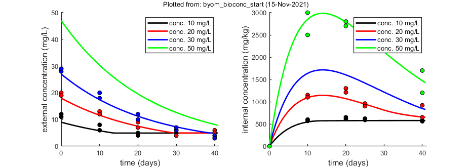
The model: An organism is exposed to a chemical in its surrounding medium. The animal accumulates the chemical according to standard one-compartment first-order kinetics, specified by a bioconcentration factor (Piw) and an elimination rate (ke). The chemical degrades at a certain rate (kd). When the external concentration reaches a certain concentration (Ct), degradation stops. This is useful to demonstrate the events function in call_deri.m, which catches this discontuity graciously.
This script: byom_bioconc_start provides a quick and clean file for your analyses. For a more detailed example, with more explanation and more options, consult byom_bioconc_extra.m or download the BYOM manual from here.
Copyright (c) 2012-2021, Tjalling Jager, all rights reserved.
This source code is licensed under the MIT-style license found in the
LICENSE.txt file in the root directory of BYOM.
Contents
Initial things
Make sure that this script is in a directory somewhere below the BYOM folder.
clear, clear global % clear the workspace and globals
global DATA W X0mat % make the data set and initial states global variables
global glo          % allow for global parameters in structure glo
diary off           % turn off the diary function (if it is accidentaly on)
% set(0,'DefaultFigureWindowStyle','docked'); % collect all figure into one window with tab controls
set(0,'DefaultFigureWindowStyle','normal'); % separate figure windows

pathdefine(0) % set path to the BYOM/engine directory (option 1 uses parallel toolbox)
glo.basenm  = mfilename; % remember the filename for THIS file for the plots
glo.saveplt = 0; % save all plots as (1) Matlab figures, (2) JPEG file or (3) PDF (see all_options.txt)
The data set
Data are entered in matrix form, time in rows, scenarios (exposure concentrations) in columns. First column are the exposure times, first row are the concentrations or scenario numbers. The number in the top left of the matrix indicates how to calculate the likelihood:
- -1 for multinomial likelihood (for survival data)
- 0 for log-transform the data, then normal likelihood
- 0.5 for square-root transform the data, then normal likelihood
- 1 for no transformation of the data, then normal likelihood
% observed external concentrations (two series per concentration)
DATA{1} = [ 1  10 10 20 20 30 30
            0  11 12 20 19 28 29
            10  6  8 13 12 20 18
            20  4  5  9  7 10 12
            30  5  7  6  4  6  7
            40  4  5  6  5  4  3];

% weight factors (number of replicates per observation in DATA{1})
W{1} = [10 10 10 10 10 10
        10 10 10 10 10 10
         8  8  8  8  8  9
         8  7  7  8  8  9
         6  6  6  6  6  7];

% observed internal concentrations (two series per concentration)
DATA{2} = [0.5   10  10   20   20   50   50
           0    0   0    0    0    0    0
           10 570 600 1150 1100 2500 3000
           20 610 650 1300 1210 2700 2800
           25 590 620  960  900 2300 2200
           40 580 560  920  650 1200 1700];

% if weight factors are not specified, ones are assumed in start_calc.m
Initial values for the state variables
Initial states, scenarios in columns, states in rows. First row are the 'names' of all scenarios.
X0mat = [10 20 30 50    % the scenarios (here nominal concentrations)
          9 18 27 47    % initial values state 1 (actual external concentrations)
          0  0  0  0];  % initial values state 2 (internal concentrations)
Initial values for the model parameters
Model parameters are part of a 'structure' for easy reference.
% syntax: par.name = [startvalue fit(0/1) minval maxval];
par.kd    = [0.1  1 0 100];  % degradation rate constant, d-1
par.ke    = [0.2  1 0 100];  % elimination rate constant, d-1
par.Piw   = [200  1 0 1e6];  % bioconcentration factor, L/kg
par.Ct    = [5    0 0 1e6];  % threshold external concentration where degradation stops, mg/L
Time vector and labels for plots
Specify what to plot. If time vector glo.t is not specified, a default is constructed, based on the data set.
% specify the y-axis labels for each state variable
glo.ylab{1} = 'external concentration (mg/L)';
glo.ylab{2} = 'internal concentration (mg/kg)';
% specify the x-axis label (same for all states)
glo.xlab    = 'time (days)';
glo.leglab1 = 'conc. '; % legend label before the 'scenario' number
glo.leglab2 = 'mg/L';   % legend label after the 'scenario' number

prelim_checks % script to perform some preliminary checks and set things up
% Note: prelim_checks also fills all the options (opt_...) with defauls, so
% modify options after this call, if needed.
Calculations and plotting
Here, the functions are called that will do the calculation and the plotting.
Options for the plotting can be set using opt_plot (see prelim_checks.m). Options for the optimsation routine can be set using opt_optim. Options for the ODE solver are part of the global glo. For the demo, the iterations were turned off (opt_optim.it = 0).
opt_optim.fit = 1; % fit the parameters (1), or don't (0)
opt_optim.it  = 0; % show iterations of the optimisation (1, default) or not (0)

% optimise and plot (fitted parameters in par_out)
par_out = calc_optim(par,opt_optim); % start the optimisation
calc_and_plot(par_out,opt_plot);     % calculate model lines and plot them
Goodness-of-fit measures for each state and each data set (R-square)
Based on the individual replicates, accounting for transformations, and including t=0
state 1.   0.96
state 2.   0.99
=================================================================================
Results of the parameter estimation with BYOM version 6.0 BETA 6
=================================================================================
   Filename      : byom_bioconc_start
   Analysis date : 15-Nov-2021 (14:48)
   Data entered  :
     data state 1: 5x6, continuous data, no transf.
     data state 2: 5x6, continuous data, power 0.50 transf.
   Search method: Nelder-Mead simplex direct search, 2 rounds.
     The optimisation routine has converged to a solution
     Total 195 simplex iterations used to optimise.
     Minus log-likelihood has reached the value 223.31 (AIC=452.61).
=================================================================================
kd        0.04381 (fit: 1, initial: 0.1)
ke         0.1099 (fit: 1, initial: 0.2)
Piw         116.9 (fit: 1, initial: 200)
Ct              5 (fit: 0, initial:  5)
=================================================================================
Time required: 3.5 secs
Plots result from the optimised parameter values.
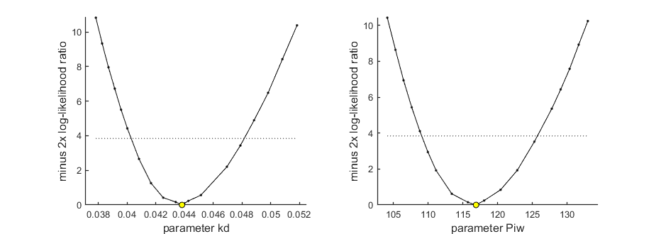
Profiling the likelihood
By profiling you make robust confidence intervals for one or more of your parameters. Use the names of the parameters as they occurs in your parameter structure par above. This can be a single string (e.g., 'kd'), a cell array of strings (e.g., {'kd','ke'}), or 'all' to profile all fitted parameters. This example produces a profile for two parameters and provides the 95% confidence interval (on screen and indicated by the horizontal broken line in the plot).
Note: for more post-calculations, see byom_bioconc_extra.m
Options for profiling can be set using opt_prof (see prelim_checks.m).
opt_prof.detail   = 2; % detailed (1) or a coarse (2) calculation
opt_prof.subopt   = 0; % number of sub-optimisations to perform to increase robustness

% UNCOMMENT LINE(S) TO CALCULATE
par_better = calc_proflik(par_out,{'kd','Piw'},opt_prof,opt_optim);  % calculate a profile
if ~isempty(par_better)                 % if the profiling found a better optimum ...
    calc_and_plot(par_better,opt_plot); % calculate model lines and plot them
end
95% confidence interval(s) from the profile(s)
=================================================================================
kd         interval:    0.04027 -  0.04814
Piw        interval:      109.1 -  125.7
=================================================================================

Time required: 48.2 secs